2 Base R (I) & 輔助工具
2.1 R Studio
2.1.1 自訂樣式
- RStudio 預設有 4 個區塊 (Pane)。你可以自行決定這 4 個區塊的位置
-
Tools–>Global Options...–> (在左欄選擇)Pane Layout - Source, Console, 及 2 個自訂區塊
-
- 除了區塊的相對位置,也可以設定 RStudio 整體的風格以及程式碼 Syntax Highlighting 的樣式:
-
Tools–>Global Options...–> (在左欄選擇)Appearance
-
2.2 函數
get_area <- function() {
    area <- 3.14 * 1 * 1
    return(area)
}
get_area()
#> [1] 3.14
# Function with a argument
get_area <- function(r) {
    area <- 3.14 * r * r
    return(area)
}
get_area(2)
#> [1] 12.56
# Function with a argument that has default value
get_area <- function(r = 1) {
    area <- 3.14 * r * r
    return(area)
}
get_area()
#> [1] 3.14
get_area <- function(r) {
    area <- 3.14 * r * r
    return(area)
}
area <- 100
area
get_area(1)
area
#> [1] 100
#> [1] 3.14
#> [1] 1002.3 Function Arguments
vol <- function(r, height = 1) {
    volumn <- 3.14 * r * r * height
    return(volumn)
}
vol(1, 2)
#> [1] 6.28
vol(r = 1, height = 2) # Be explicit#> [1] 6.28
# If all args are named, order doesn't matter
vol(height = 2, r = 1)
#> [1] 6.28
# Mix named and unnamed args:
# named args will be assigned first, then
# unnamed args will be assigned
# based on their positions
vol(height = 2, 1)
#> [1] 6.282.4 vector
-
上週實習課使用 R 時,指令的回傳值多半只有「一個」。但 R 其實是一種以向量作為基本單位的程式語言,所以對於「一個回傳值」更精確的描述應該是「一個長度為 1 的向量」。
x <- 2
x
#> [1] 2is.vector(x)#> [1] TRUElength(x)#> [1] 1 -
我們上週簡短提過以
:製造數列的方式 (e.g.1:10)。事實上,這個回傳的數列即是一個 vector。另外,由於這個 vector 的每個元素皆是整數,因此這個 vector 屬於 integer vector。我們可以使用typeof()確認 vector 的類別typeof(1:10)#> [1] "integer" R 裡面的 vector 可以被分成 6 種類別,其中常見的 4 種分別為
integer,double, ,character,logical
2.4.1 integer vector
- integer vector 的元素由整數組成,它可以是零、正或負的。除了使用
:製造數列,也可以使用c()(稱為 concatenate) 組出任意序列的 vector。- 使用
c()製造 integer vector 時,每個整數數字後面必須接L,若沒有加上L, R 會將製造出來的 vector 視為 double vector。
- 使用
#> [1] -1 5 2
dbl_vec#> [1] -1 5 2
typeof(int_vec)#> [1] "integer"
typeof(dbl_vec)#> [1] "double"2.4.2 double vector
double vector 儲存的是浮點數,亦即含有小數點的數字 (e.g
1.2,-0.75)-
在 R 裡面,integer vector 與 double vector 合稱為 numeric vector,兩者之間的區隔通常也不太重要,因為 R 在運算時,通常會將這兩種資料類型自動轉換成合適的類型
typeof(2L)#> [1] "integer"typeof(2.0)#> [1] "double"is.numeric(2L)#> [1] TRUEis.numeric(2.0)#> [1] TRUEtypeof(1L + 1.0)#> [1] "double"typeof(1L / 2L)#> [1] "double" -
Special values:
Inf: 代表無限大-
NaN: “Not a Number”,常見於數字運算不符數學定義時,例如:0 / 0#> [1] NaNInf / Inf#> [1] NaNlog(-1)#> Warning in log(-1): NaNs produced#> [1] NaN
2.4.3 character vector
-
除了數字以外,R 也可以儲存字串 (string)。character vector 的每個元素皆由一個字串所組成。在 R 裡面,只要是被引號 (quote,
'或"皆可) 包裹的東西就是字串,放在引號內的可以是任何字元 (e.g. 空白、數字、中文字、英文字母)"1.1" # This is a string (character vector of length 1), not double#> [1] "1.1""你好!"#> [1] "你好!"c("1.1", "你好!")#> [1] "1.1" "你好!" -
如果字串內含有引號
",需在字串內的引號前使用跳脫字元\,以表示此引號是字串的一部分而非字串的開頭或結尾- 或是,你可以使用「不同的」引號。例如以「單引號」表示字串的開頭與結尾時,字串內就可以直接使用「雙引號」,反之亦然
"\""  # escape a double quote
'\''  # escape a single quote
'"'   # a double quote as string without escaping
"'"   # a single quote as string without escaping
#> [1] "\"" #> [1] "'" #> [1] "\"" #> [1] "'"
2.4.4 logical vector
logical vector 的每個元素由
TRUE或FALSE組成。可以使用
c()一項項手動輸入製造 logical vector-
logical vector 的另一個來源則是 logical test 的回傳值:
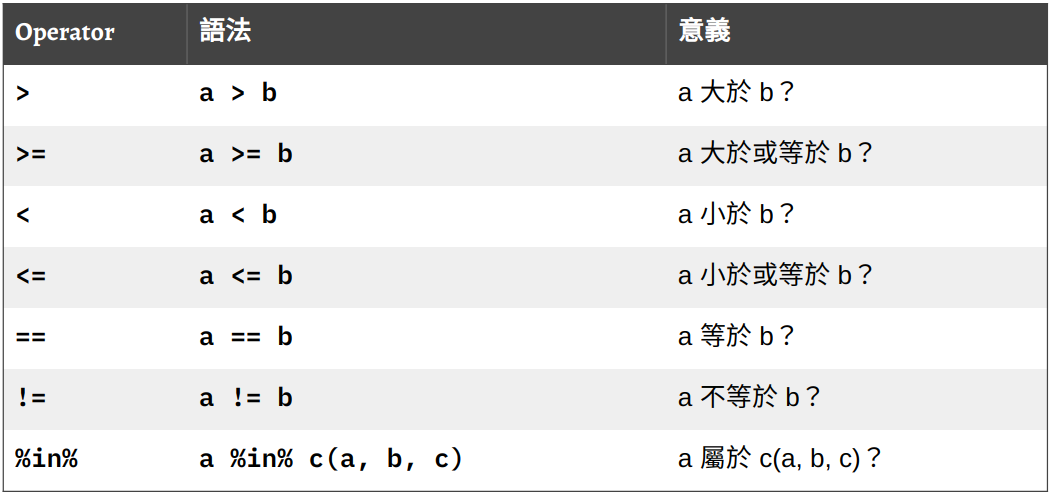
# logical tests
vec1 > vec2
#> [1] FALSE TRUE FALSEvec1 < vec2#> [1] TRUE FALSE TRUEvec1 == vec2#> [1] FALSE FALSE FALSE -
boolean operators (
&,|,!,any(),all()) 可以整合多個 logical tests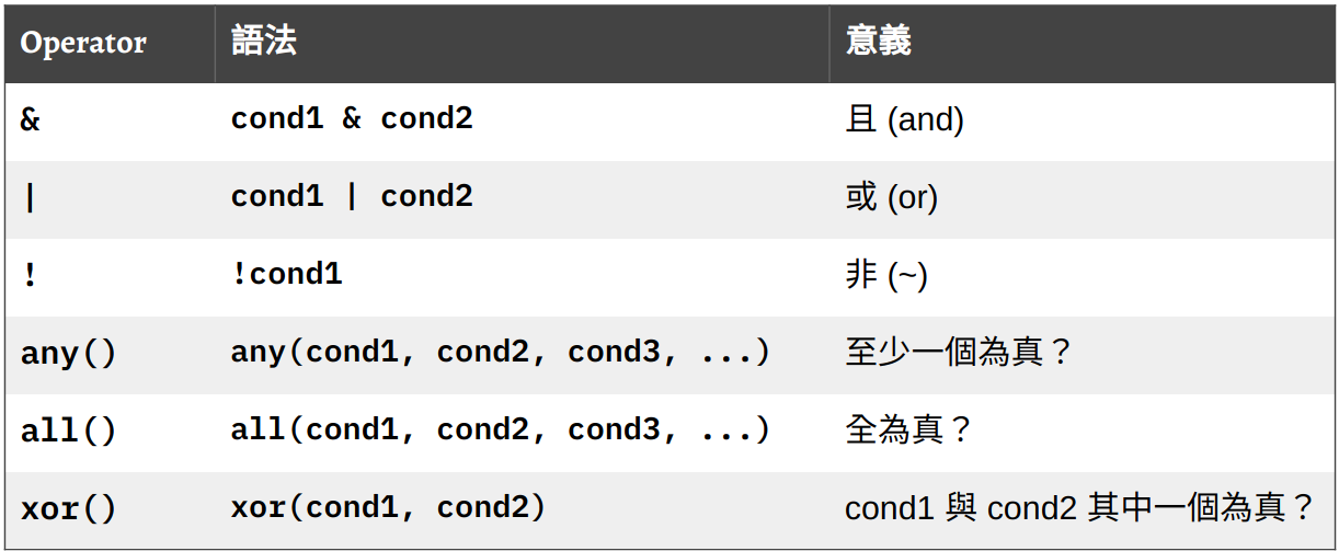
TRUE & TRUE#> [1] TRUETRUE & FALSE#> [1] FALSETRUE | FALSE#> [1] TRUE!TRUE#> [1] FALSE(1 == 1) & (2 == 2)#> [1] TRUE
2.5 Recycling
- 兩個或兩個以上的 vector 進行運算時,通常是以 element-wise 的方式進行。此時,若進行運算的 vector 長度不相同,例如,
c(1, 2, 3) + 2, R 會自動將長度較短 vector (2) 「回收 (recycle)」,亦即,重複此向量內的元素使其「拉長」到與另一個 vector 等長;接著再將兩個一樣長的 vector 進行 element-wise 的向量運算。
x <- c(1, 1, 2, 2)

# Arithmetic operation
x + 2  # equivalent to...
#> [1] 3 3 4 4
x + c(2, 2, 2, 2)#> [1] 3 3 4 4
x <- c(1, 1, 2, 2)

# Logical operation
x == 2  # equivalent to...
#> [1] FALSE FALSE TRUE TRUE
x == c(2, 2, 2, 2)#> [1] FALSE FALSE TRUE TRUE#> [1] "a1"
paste0(long, short)#> [1] "a1" "b1" "c1"2.6 Coercion
vector 內的每個元素,其資料類型 (data type) 必須相同。資料類型即是前面提到的
integer,double,character,logical。-
若發生資料類型不一致的情形 (e.g. 將不同資料類型的元素放入
c()),R 會根據某些規則,自動進行資料類型的轉換。這個過程在 R 裡面稱為 Coercionc(TRUE, FALSE, 3) # logical & numeric#> [1] 1 0 3c(-1, "aa") # numeric & character#> [1] "-1" "aa"c(FALSE, TRUE, "hi!") # logical & character#> [1] "FALSE" "TRUE" "hi!"c(TRUE, 0, "hi!") # logical & numeric & character#> [1] "TRUE" "0" "hi!"
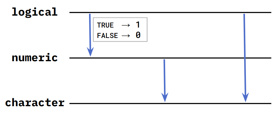
Figure 2.1: Rules of Coercion
if coercion failed, throw error
manual coercion:
as.character(),as.logical(),as.numeric()
#> [1] 3#> [1] 2
mean(gender == "male") # proportion of male#> [1] 0.52.7 Subsetting a vector
- 有 3 種方法可用於取出 vector 裡面的元素 (回傳一個新的 vector)
- 透過提供 vector 中元素的位置次序 (index)
- 透過一個與此 vector 等長的 logical vector。在 logical vector 中的相對應位置,以
TRUE或FALSE表示是否保留該位置的元素 - 透過提供元素的「名字」(i.e.
names屬性)
2.7.1 index subsetting
# z[<integer_vector>]
LETTERS  # R 內建變數: 包含所有大寫英文字母的 character vector
#> [1] "A" "B" "C" "D" "E" "F" "G" "H" "I" "J" "K" "L" "M" "N" "O" "P" "Q" "R" "S"
#> [20] "T" "U" "V" "W" "X" "Y" "Z"
LETTERS[1]#> [1] "A"
LETTERS[1:5]#> [1] "A" "B" "C" "D" "E"
LETTERS[c(1, 3, 5)]#> [1] "A" "C" "E"
LETTERS[-(1:5)] # Exclude the first 5 elements#> [1] "F" "G" "H" "I" "J" "K" "L" "M" "N" "O" "P" "Q" "R" "S" "T" "U" "V" "W" "X"
#> [20] "Y" "Z"2.7.2 Logical subsetting
#> [1] 20 19
## Creating logical vectors
age[1] < 20  # returns a logical vector of length 1
#> [1] FALSE
age < 20 # returns a logical vector of length(x)#> [1] FALSE FALSE TRUE TRUE
# Subset a vector using a logical test
age[age < 20]
#> [1] 18 192.7.3 Subsetting with names
age <- c(40, 20, 18, 19)
names(age) <- c("kai", "pooh", "tiger", "piglet")
# age <- c(kai = 40, pooh = 20, tiger = 18, piglet = 19)  # another way of setting names

age
#> kai pooh tiger piglet
#> 40 20 18 19
age['kai'] + 9#> kai
#> 49
age[c('pooh', 'kai')]#> pooh kai
#> 20 402.7.4 Modifying Values in vector
a2z <- LETTERS
a2z[1:3] <- c("a", "b", "c")
a2z
#> [1] "a" "b" "c" "D" "E" "F" "G" "H" "I" "J" "K" "L" "M" "N" "O" "P" "Q" "R" "S"
#> [20] "T" "U" "V" "W" "X" "Y" "Z"
gender <- c("m", "m", "f", "f")
gender[gender == "m"] <- "male"
gender
#> [1] "male" "male" "f" "f"
gender[gender == "f"] <- "female"
gender
#> [1] "male" "male" "female" "female"#> john jenny jane kate
#> "male" "male" "female" "female"
gender["john"] <- "male"
gender
#> john jenny jane kate
#> "male" "male" "female" "female"
gender[c("jenny", "jane", "kate")] <- "female"
gender
#> john jenny jane kate
#> "male" "female" "female" "female"2.8 if else
- 一般而言,R 是由上至下一行一行地執行程式碼。有時候我們會希望能跳過某些程式碼或是依據不同的狀況執行不同的程式碼,這時候我們就需要使用條件式。
#> [1] "x is positive"
x <- -1

if (x > 0) {
    print('x is positive')
} else if (x < 0) {
    print('x is negative')
} else {
    print('x is zero')
}

print('This is always printed')
#> [1] "x is negative"
#> [1] "This is always printed"在
if-else if-else的結構中,只有其中一個區塊 (被大括弧{}包裹的程式碼) 會被執行。執行完該區塊後,就會忽略剩下的條件控制區塊,執行條件式之後的程式碼。可以在
if之後使用多個else if.-
條件式的結構:
# 只有 if
if (<條件>) {
    <Some Code>  # 條件成立時執行
}

# if, else
if (<條件>) {
    <Some Code>  # <條件>成立時執行
} else {
    <Some Code>  # <條件>不成立時執行
}

# if, else if, else
if (<條件1>) {
    <Some Code>          # <條件1>成立時執行
} else if ( <條件2> ) {
    <Some Code>          # <條件1>不成立、<條件2>成立時執行
} else {
    <Some Code>          # <條件1>、<條件2>皆不成立時執行
}
2.9 Wrap up: 句子產生器
# Data
name <- c("kai", "pooh", "tiger", "piglet")
age <- c(40, 20, 18, 19)

# Randomly draw 2 subjects
who <- sample(1:4, size = 2)

# Find out who is older
age1 <- age[who[1]]
age2 <- age[who[2]]
if (age1 > age2) {
    comparitive <- ' is older than '
} else if (age1 < age2) {
    comparitive <- ' is younger than '
} else {
    comparitive <- ' is as old as '
}

# Construct sentence
paste0(name[who[1]], comparitive, name[who[2]])
#> [1] "piglet is younger than kai"2.10 R Markdown
-
使用前需先安裝
rmarkdown:install.packages('rmarkdown') R Markdown (
.Rmd) 就像之前同學用來寫自我介紹的 Markdown 文件 (.md) 一樣是一種純文字格式。R Markdown 的語法其實只是 Markdown 的一種擴充:它新增了一些特殊的語法,讓使用者可以直接在 R Markdown 裡面撰寫程式碼,並透過 R 將這些程式碼的運算結果插入 R Markdown 的輸出文件當中。-
knitr Code Chunk
- 執行:由上至下執行
- 後面的 chunk 可以讀取之前的 chunks 產生的變數
(在 RStudio 使用 R Markdown)
使用 RStudio 開啟 R Markdown (
.Rmd) 時,Rmd 檔會出現在 Source Pane 讓使用者編輯將 R Markdown (
.Rmd) 輸出 (knit)成 HTML 檔 (.html):
![R Markdown document in RStudio^[Figure from https://bookdown.org/yihui/rmarkdown/images/hello-rmd.png].](https://bookdown.org/yihui/rmarkdown/images/hello-rmd.png)
Figure 2.2: R Markdown document in RStudio10.
參考資源
Grolemund, G. (2014). Hands-on programming with R
R Objects (https://rstudio-education.github.io/hopr/r-objects)
Modifying Values (https://rstudio-education.github.io/hopr/modify)Xie, Y., Allaire, J., & Grolemund, G. (2019). R Markdown: The Definitive Guide